Performance Analysis of VersionedHDF5 Files: File sizes

For these tests, we have generated .h5 data files using the generate_data.py script from the VersionedHDF5 repository, using the standard options (see more details in Performance.)

We performed the following tests:

1. Test Large Fraction Changes Sparse

2. Test Mostly Appends Sparse

3. Test Small Fraction Changes Sparse

4. Test Large Fraction Changes (Constant Array Size) Sparse

5. Test Mostly Appends Dense

Setup

import h5py
import json
import numpy as np
import performance_tests
import matplotlib.pyplot as plt

The information from the generated test files are stored in either

• testcase.tests, a dictionary containing all the info related to a testcase that was run recently;

• a .json file named after the test name and options, containing a summary of the results. This file can be read with

with open("<filename>.json", "r") as json_in:
      test = json.load(json_in)

Test 1: Large fraction changes (sparse)

testname = "test_large_fraction_changes_sparse"

For the number of transactions, chunk sizes and compression algorithms, we tests the following options:

num_transactions_1 = [50, 100, 500, 1000, 5000]
exponents_1 = [12, 14]
compression_1 = [None, "gzip", "lzf"]

(note that chunk sizes are taken as power of 2, so an exponent of \(12\) means that the chunk size is \(2^12\) or 4096.)

If you want to generate your own tests, you can modify the appropriate constants for the desired tests, and run them on the notebook included in the analysis directory of the VersionedHDF souces. Please keep in mind that file sizes can become very large for large numbers of transactions (above 5000 transactions).

Analysis

First, let’s obtain some common parameters from the tests:

num_transactions = [test['num_transactions'] for test in testcase_1]
chunk_sizes = [test['chunk_size'] for test in testcase_1]
compression = [test['compression'] for test in testcase_1]
filesizes = np.array([test['size'] for test in testcase_1])
sizelabels = np.array([test['size_label'] for test in testcase_1])
max_no_versions = max(np.array([test['size'] for test in testcase_1_no_versions]))

n = len(set(num_transactions))
ncs = len(set(chunk_sizes))
ncomp = len(set(compression))

We’ll start by analyzing how the .h5 file sizes grow as the number of versions grows.

Note that the array size also can also grow as the number of versions grows, since each transaction is changing the original arrays by adding, deleting and changing values in the original arrays. In order to compute a (naive) theoretical lower bound on the file size, we can compute how much space each version should take. However, this does not account for overhead and particular details of chunking. Keep in mind there is redundant data as some of it is not changed during the staging of a new version but it is still being stored.

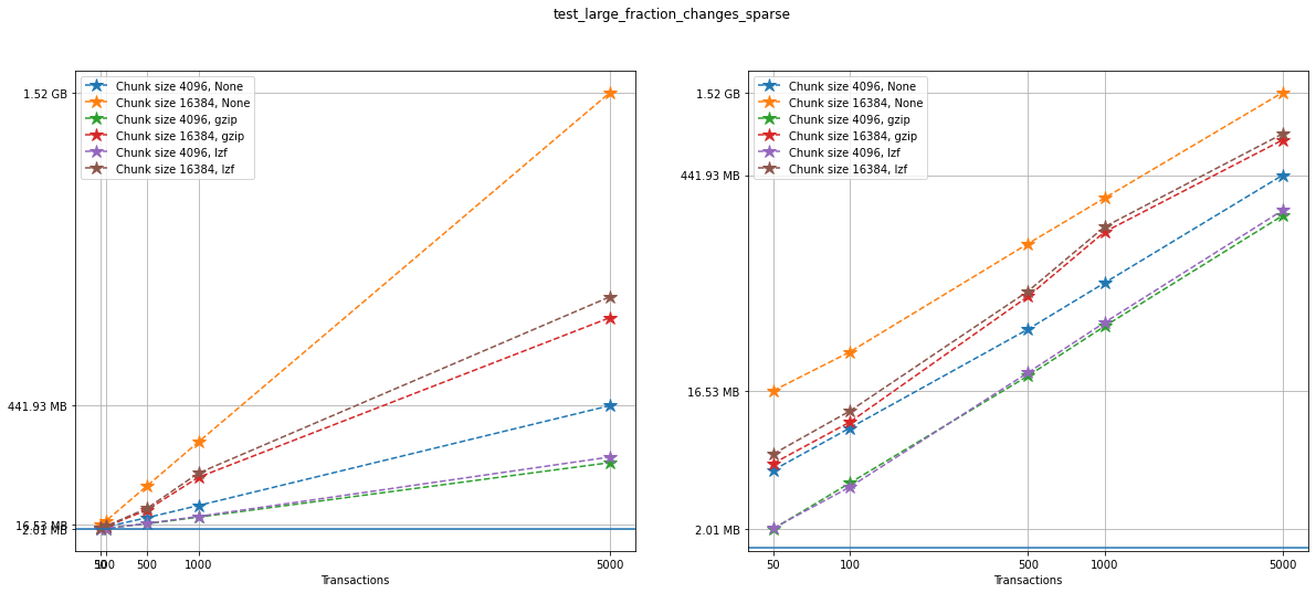
Let’s show the size information in a plot. On the left, we can see a linear plot, and on the right a loglog plot of the same size data for testcase_1. On the bottom, a blue solid horizontal line indicates the maximum file size obtained when generating the same tests with no versioning (that is, not using VersionedHDF5).

fig, ax = plt.subplots(nrows=1, ncols=2, figsize=(20,8))

# Changing the indices in selected will change the y-axis ticks in the graph for better visualization
selected = [4, 5, 9, 10]

for i in range(ncomp):
    start = i*ncs*n
    for j in range(ncs):
        ax[0].plot(num_transactions[:n],
                   filesizes[start+j*n:start+(j+1)*n],
                   '*--', ms=12,
                   label=f"Chunk size {chunk_sizes[start+j*n]}, {compression[start]}")
        ax[1].loglog(num_transactions[:n],
                     filesizes[start+j*n:start+(j+1)*n],
                     '*--', ms=12,
                     label=f"Chunk size {chunk_sizes[start+j*n]}, {compression[start]}")
        ax[0].legend(loc='upper left')
        ax[1].legend(loc='upper left')
        ax[0].minorticks_off()
        ax[1].minorticks_off()
        ax[0].set_xticks(num_transactions[:n])
        ax[0].set_xticklabels(num_transactions[:n])
        ax[0].set_yticks(filesizes[selected])
        ax[0].set_yticklabels(sizelabels[selected])
        ax[0].set_xlabel("Transactions")
        ax[0].grid(True)
        ax[1].set_xticks(num_transactions[:n])
        ax[1].set_xticklabels(num_transactions[:n])
        ax[1].set_yticks(filesizes[selected])
        ax[1].set_yticklabels(sizelabels[selected])
        ax[1].set_xlabel("Transactions")
        ax[1].grid(True)

ax[0].axhline(max_no_versions)
ax[1].axhline(max_no_versions)
plt.suptitle(f"{testname}")
plt.show()

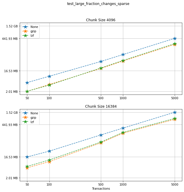
Comparing compression algorithms

For each chunk size that we chose to test, let’s compare the file sizes corresponding to each compression algorithm that we used.

fig, ax = plt.subplots(ncs, figsize=(10,10), sharey=True)
fig.suptitle(f"{testname}: File sizes")

for i in range(ncomp):
    start = i*ncs*n
    for j in range(ncs):
        ax[j].loglog(num_transactions[:n],
                     filesizes[start+j*n:start+(j+1)*n],
                     '*--', ms=12,
                     label=f"{compression[start]}")
        ax[j].legend(loc='upper left')
        ax[j].set_title(f"Chunk Size {chunk_sizes[start+j*n]}")
        ax[j].set_xticks(num_transactions[:n])
        ax[j].set_xticklabels(num_transactions[:n])
        ax[j].set_yticks(filesizes[selected])
        ax[j].set_yticklabels(sizelabels[selected])
        ax[j].grid(True)
        ax[j].minorticks_off()

plt.xlabel("Transactions")
plt.suptitle(f"{testname}")
plt.show()

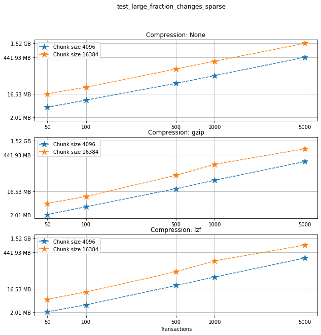
Comparing chunk sizes

Now, for each choice of compression algorithm, we compare different chunk sizes.

fig, ax = plt.subplots(ncomp, figsize=(10,10), sharey=True)
fig.suptitle(f"{testname}: File sizes")

for i in range(ncomp):
    start = i*ncs*n
    for j in range(ncs):
        plotlabel = f"Chunk size {chunk_sizes[start+j*n]}"
        plottitle = f"Compression: {compression[start]}"
        ax[i].loglog(num_transactions[:n],
                     filesizes[start+j*n:start+(j+1)*n],
                     '*--', ms=12,
                     label=plotlabel)
        ax[i].legend(loc='upper left')
        ax[i].set_title(plottitle)
        ax[i].set_xticks(num_transactions[:n])
        ax[i].set_xticklabels(num_transactions[:n])
        ax[i].set_yticks(filesizes[selected])
        ax[i].set_yticklabels(sizelabels[selected])
        ax[i].grid(True)
        ax[i].minorticks_off()

plt.xlabel("Transactions")
plt.suptitle(f"{testname}")
plt.show()

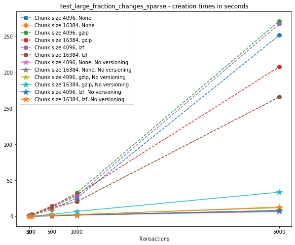
Creation times

If we look at the creation times for these files, we have something like this:

t_write = np.array([test['t_write'][-1] for test in testcase_1])
fig_large_fraction_changes_times = plt.figure(figsize=(10,8))
for i in range(ncomp):
    start = i*ncs*n
    for j in range(ncs):
        plt.plot(num_transactions[:n],
                 t_write[start+j*n:start+(j+1)*n],
                 'o--', ms=8,
                 label=f"Chunk size {chunk_sizes[start+j*n]}, {compression[start]}")

# If you also with to plot information about the "no versions" test,
# run the following lines:
t_write_nv = np.array([test['t_write'][-1] for test in testcase_1_no_versions])
for i in range(ncomp):
    start = i*ncs*n
    for j in range(ncs):
        plt.plot(num_transactions[:n],
                 t_write_nv[start+j*n:start+(j+1)*n],
                 '*-', ms=12,
                 label=f"Chunk size {chunk_sizes[start+j*n]}, {compression[start]}, No versioning")

plt.xlabel("Transactions")
plt.title(f"{testname} - creation times in seconds")
plt.legend()
plt.xticks(num_transactions[:n])
plt.show()

Now, we can look at the time required to stage a new version in the file, that is, to add a new transaction. The graphs below show, for each fixed number of transactions, the time required to add new versions as the file is created.

fig_times, ax = plt.subplots(n+1, figsize=(14,20))
fig_times.suptitle(f"{testname}: time to write each new version")

for i in range(n):
    for test in testcase_1:
        if test['num_transactions'] == num_transactions[i]:
            t_write = np.array(test['t_write'][:-1])
            ax[i].plot(t_write,
                       label=f"chunk size {test['chunk_size']}, {test['compression']}")
            ax[i].legend(loc='upper left')

# If you also with to plot information about the "no versions" test,
# run the following lines:
for test in testcase_1_no_versions:
    if test['num_transactions'] == num_transactions[i]:
        t_write = np.array(test['t_write'][:-1])
        ax[n].plot(t_write,
                   label=f"chunk size {test['chunk_size']}, {test['compression']}")
        ax[n].legend(loc='upper left')
        ax[n].set_title('No versioning')

plt.xlabel("Number of transactions")
plt.ylabel("Time (in seconds)")
plt.show()

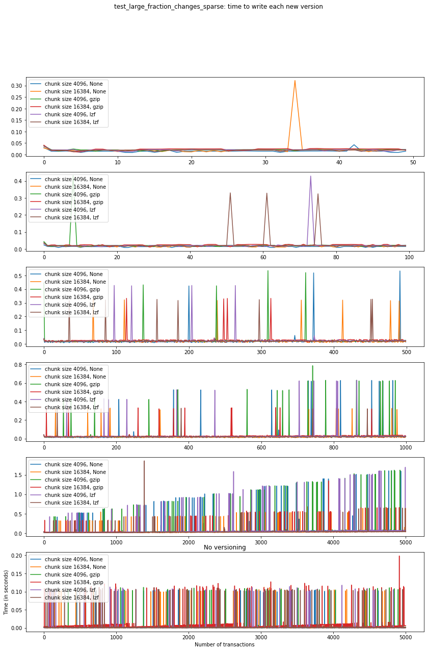
Summary

We can clearly see that files with smallest file size, corresponding to smaller chunk sizes, are also the ones with largest creation times. This is consistent with the effects of using smaller chunk sizes in HDF5 files.

This behaviour suggests that for test_large_fraction_changes_sparse, larger chunk sizes generate larger files, but the size of the files grows as expected as the number of transactions grow. So, if we are dealing with a large number of transactions, larger chunk sizes generate files that are larger while having faster creation times (and probably faster read/write speeds as well).

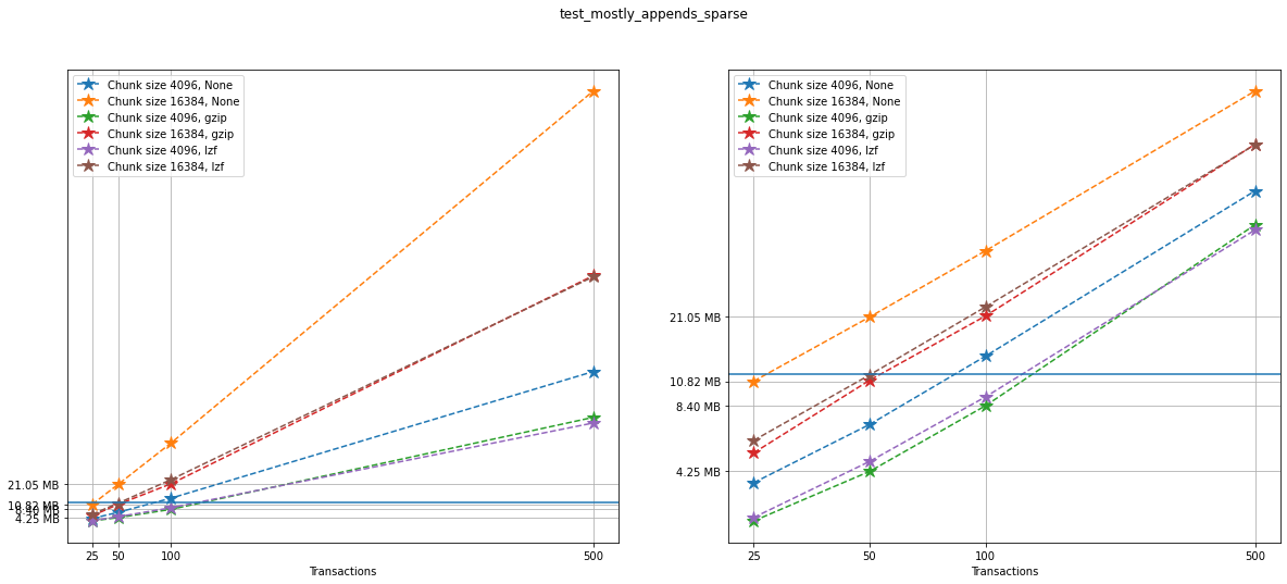
Test 2: Mostly appends (sparse)

testname = "test_mostly_appends_sparse"

For this case, we have tested the following options:

num_transactions_2 = [25, 50, 100, 500]
exponents_2 = [12, 14]
compression_2 = [None, "gzip", "lzf"]

Analysis

Repeating the same analysis as in the previous test, let’s show the size information in a graph:

num_transactions = [test['num_transactions'] for test in testcase_2]
chunk_sizes = [test['chunk_size'] for test in testcase_2]
compression = [test['compression'] for test in testcase_2]
filesizes = np.array([test['size'] for test in testcase_2])
sizelabels = np.array([test['size_label'] for test in testcase_2])
max_no_versions = max(np.array([test['size'] for test in testcase_2_no_versions]))

n = len(set(num_transactions))
ncs = len(set(chunk_sizes))
ncomp = len(set(compression))

Similarly to what we did before, on the left we can see a linear plot, and on the right a loglog plot of the same size data for testcase_2. A blue solid horizontal line indicates the maximum file size obtained when generating the same tests with no versioning (that is, not using VersionedHDF5).

fig, ax = plt.subplots(nrows=1, ncols=2, figsize=(20,8))

selected = [4, 5, 9, 10]

for i in range(ncomp):
    start = i*ncs*n
    for j in range(ncs):
        ax[0].plot(num_transactions[:n],
                   filesizes[start+j*n:start+(j+1)*n],
                   '*--', ms=12,
                   label=f"Chunk size {chunk_sizes[start+j*n]}, {compression[start]}")
        ax[1].loglog(num_transactions[:n],
                     filesizes[start+j*n:start+(j+1)*n],
                     '*--', ms=12,
                     label=f"Chunk size {chunk_sizes[start+j*n]}, {compression[start]}")
        ax[0].legend(loc='upper left')
        ax[1].legend(loc='upper left')
        ax[0].minorticks_off()
        ax[1].minorticks_off()
        # Changing the indices in selected will change the y-axis ticks in the graph for better visualization
        ax[0].set_xticks(num_transactions[:n])
        ax[0].set_xticklabels(num_transactions[:n])
        ax[0].set_yticks(filesizes[selected])
        ax[0].set_yticklabels(sizelabels[selected])
        ax[0].set_xlabel("Transactions")
        ax[0].grid(True)
        ax[1].set_xticks(num_transactions[:n])
        ax[1].set_xticklabels(num_transactions[:n])
        ax[1].set_yticks(filesizes[selected])
        ax[1].set_yticklabels(sizelabels[selected])
        ax[1].set_xlabel("Transactions")
        ax[1].grid(True)

ax[0].axhline(max_no_versions)
ax[1].axhline(max_no_versions)
plt.suptitle(f"{testname}")
plt.show()

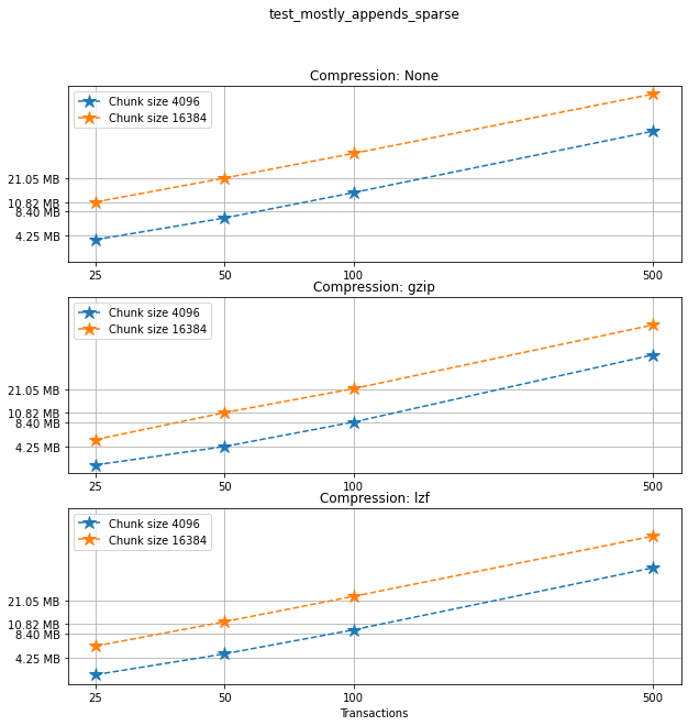
Comparing compression algorithms

For each chunk size that we chose to test, let’s compare the file sizes corresponding to each compression algorithm that we used.

fig, ax = plt.subplots(ncs, figsize=(10,10), sharey=True)
fig.suptitle(f"{testname}: File sizes")

for i in range(ncomp):
    start = i*ncs*n
    for j in range(ncs):
        ax[j].loglog(num_transactions[:n],
                     filesizes[start+j*n:start+(j+1)*n],
                     '*--', ms=12,
                     label=f"{compression[start]}")
        ax[j].legend(loc='upper left')
        ax[j].set_title(f"Chunk Size {chunk_sizes[start+j*n]}")
        ax[j].set_xticks(num_transactions[:n])
        ax[j].set_xticklabels(num_transactions[:n])
        ax[j].set_yticks(filesizes[selected])
        ax[j].set_yticklabels(sizelabels[selected])
        ax[j].grid(True)
        ax[j].minorticks_off()

plt.xlabel("Transactions")
plt.suptitle(f"{testname}")
plt.show()

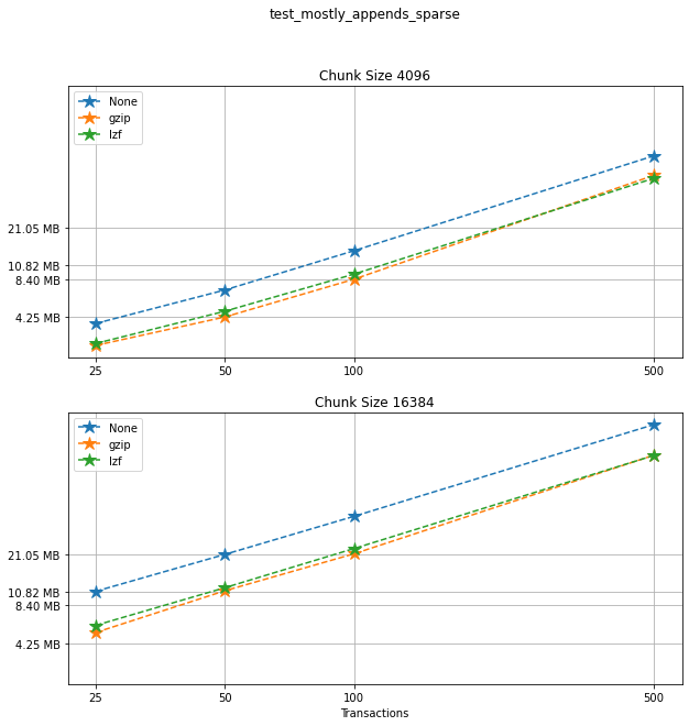
Comparing chunk sizes

Now, for each choice of compression algorithm, we compare different chunk sizes.

fig, ax = plt.subplots(ncomp, figsize=(10,10), sharey=True)
fig.suptitle(f"{testname}: File sizes")

for i in range(ncomp):
    start = i*ncs*n
    for j in range(ncs):
        plotlabel = f"Chunk size {chunk_sizes[start+j*n]}"
        plottitle = f"Compression: {compression[start]}"
        ax[i].loglog(num_transactions[:n],
                     filesizes[start+j*n:start+(j+1)*n],
                     '*--', ms=12,
                     label=plotlabel)
        ax[i].legend(loc='upper left')
        ax[i].set_title(plottitle)
        ax[i].set_xticks(num_transactions[:n])
        ax[i].set_xticklabels(num_transactions[:n])
        ax[i].set_yticks(filesizes[selected])
        ax[i].set_yticklabels(sizelabels[selected])
        ax[i].grid(True)
        ax[i].minorticks_off()

plt.xlabel("Transactions")
plt.suptitle(f"{testname}")
plt.show()

Creation times

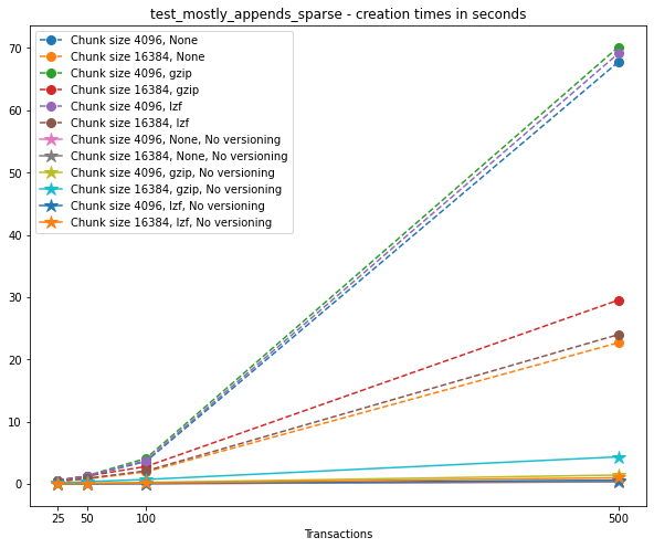
The creation times for each file are as follows.

t_write = np.array([test['t_write'][-1] for test in testcase_2])
fig_large_fraction_changes_times = plt.figure(figsize=(10,8))
for i in range(ncomp):
    start = i*ncs*n
    for j in range(ncs):
        plt.plot(num_transactions[:n],
                 t_write[start+j*n:start+(j+1)*n],
                 'o--', ms=8,
                 label=f"Chunk size {chunk_sizes[start+j*n]}, {compression[start]}")

# If you also with to plot information about the "no versions" test,
# run the following lines:
t_write_nv = np.array([test['t_write'][-1] for test in testcase_2_no_versions])
for i in range(ncomp):
    start = i*ncs*n
    for j in range(ncs):
        plt.plot(num_transactions[:n],
                 t_write_nv[start+j*n:start+(j+1)*n],
                 '*-', ms=12,
                 label=f"Chunk size {chunk_sizes[start+j*n]}, {compression[start]}, No versioning")

plt.xlabel("Transactions")
plt.title(f"{testname} - creation times in seconds")
plt.legend()
plt.xticks(num_transactions[:n])
plt.show()

Again, the graphs below show, for each fixed number of transactions, the time required to add new versions as the file is created.

fig_times, ax = plt.subplots(n+1, figsize=(14,20))
fig_times.suptitle(f"{testname}: time to write each new version")

for i in range(n):
    for test in testcase_2:
        if test['num_transactions'] == num_transactions[i]:
            t_write = np.array(test['t_write'][:-1])
            ax[i].plot(t_write,
                       label=f"chunk size {test['chunk_size']}, {test['compression']}")
            ax[i].legend(loc='upper left')

# If you also with to plot information about the "no versions" test,
# run the following lines:
for test in testcase_2_no_versions:
    if test['num_transactions'] == num_transactions[i]:
        t_write = np.array(test['t_write'][:-1])
        ax[n].plot(t_write,
                   label=f"chunk size {test['chunk_size']}, {test['compression']}")
        ax[n].legend(loc='upper left')
        ax[n].set_title('No versioning')

plt.xlabel("Number of transactions")
plt.ylabel("Time (in seconds)")
plt.show()

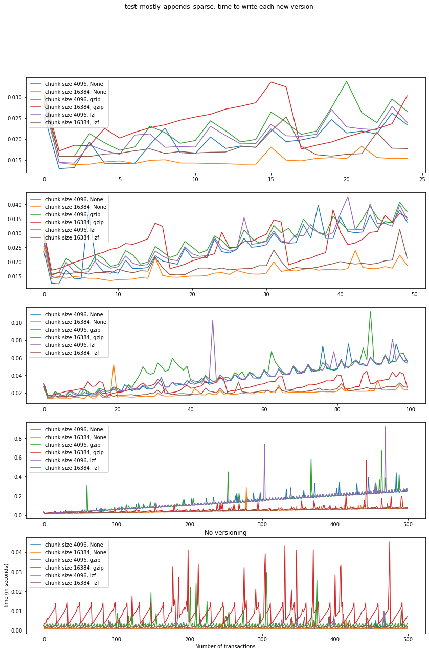
Summary

In this test, we can see that creation times are higher, which is expected since the arrays in the dataset grow significantly in size from one version to the next. Again, smaller chunk sizes correspond to smaller file sizes, but larger creation times. However, in this case, we can see there is a drop in performance when adding new versions as our file grows. This can be seen as an effect of the increase in the data size for each new version (since we are mostly appending data with each new version) but can’t be explained by that alone, as evidenced by the difference in scale between creation times for the versioned and non-versioned cases.

Test 3: Small fraction changes (sparse)

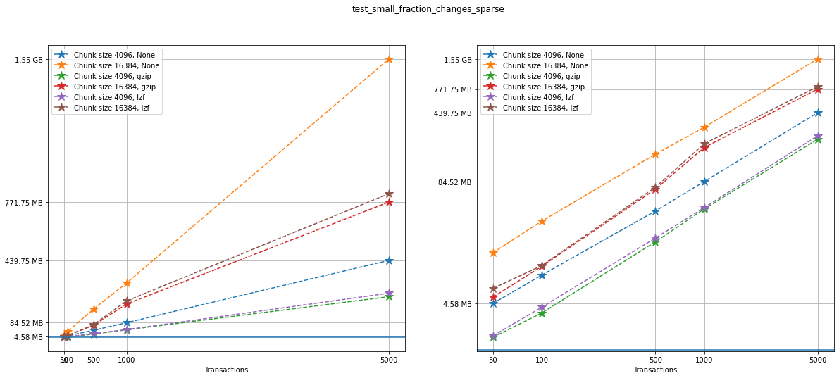
testname = "test_small_fraction_changes_sparse"

We have tested the following options:

num_transactions_3 = [50, 100, 500, 1000, 5000]
exponents_3 = [12, 14]
compression_3 = [None, "gzip", "lzf"]

Analysis

Again, let’s show the size information in a graph:

num_transactions = [test['num_transactions'] for test in testcase_3]
chunk_sizes = [test['chunk_size'] for test in testcase_3]
compression = [test['compression'] for test in testcase_3]
filesizes = np.array([test['size'] for test in testcase_3])
sizelabels = np.array([test['size_label'] for test in testcase_3])
max_no_versions = max(np.array([test['size'] for test in testcase_3_no_versions]))

n = len(set(num_transactions))
ncs = len(set(chunk_sizes))
ncomp = len(set(compression))

Again, on the left we can see a linear plot, and on the right a loglog plot of the same size data for testcase_3. A blue solid horizontal line indicates the maximum file size obtained when generating the same tests with no versioning (that is, not using VersionedHDF5).

fig, ax = plt.subplots(nrows=1, ncols=2, figsize=(20,8))

# Changing the indices in selected will change the y-axis ticks in the graph for better visualization
selected = [0, 3, 4, 9, 19]

for i in range(ncomp):
    start = i*ncs*n
    for j in range(ncs):
        ax[0].plot(num_transactions[:n],
                   filesizes[start+j*n:start+(j+1)*n],
                   '*--', ms=12,
                   label=f"Chunk size {chunk_sizes[start+j*n]}, {compression[start]}")
        ax[1].loglog(num_transactions[:n],
                     filesizes[start+j*n:start+(j+1)*n],
                     '*--', ms=12,
                     label=f"Chunk size {chunk_sizes[start+j*n]}, {compression[start]}")
        ax[0].legend(loc='upper left')
        ax[1].legend(loc='upper left')
        ax[0].minorticks_off()
        ax[1].minorticks_off()
        ax[0].set_xticks(num_transactions[:n])
        ax[0].set_xticklabels(num_transactions[:n])
        ax[0].set_yticks(filesizes[selected])
        ax[0].set_yticklabels(sizelabels[selected])
        ax[0].set_xlabel("Transactions")
        ax[0].grid(True)
        ax[1].set_xticks(num_transactions[:n])
        ax[1].set_xticklabels(num_transactions[:n])
        ax[1].set_yticks(filesizes[selected])
        ax[1].set_yticklabels(sizelabels[selected])
        ax[1].set_xlabel("Transactions")
        ax[1].grid(True)

ax[0].axhline(max_no_versions)
ax[1].axhline(max_no_versions)
plt.suptitle(f"{testname}")
plt.show()

Comparing compression algorithms

For each chunk size that we chose to test, let’s compare the file sizes corresponding to each compression algorithm that we used.

fig, ax = plt.subplots(ncs, figsize=(10,10), sharey=True)
fig.suptitle(f"{testname}: File sizes")

for i in range(ncomp):
    start = i*ncs*n
    for j in range(ncs):
        ax[j].loglog(num_transactions[:n],
                     filesizes[start+j*n:start+(j+1)*n],
                     '*--', ms=12,
                     label=f"{compression[start]}")
        ax[j].legend(loc='upper left')
        ax[j].set_title(f"Chunk Size {chunk_sizes[start+j*n]}")
        ax[j].set_xticks(num_transactions[:n])
        ax[j].set_xticklabels(num_transactions[:n])
        ax[j].set_yticks(filesizes[selected])
        ax[j].set_yticklabels(sizelabels[selected])
        ax[j].grid(True)
        ax[j].minorticks_off()

plt.xlabel("Transactions")
plt.suptitle(f"{testname}")
plt.show()

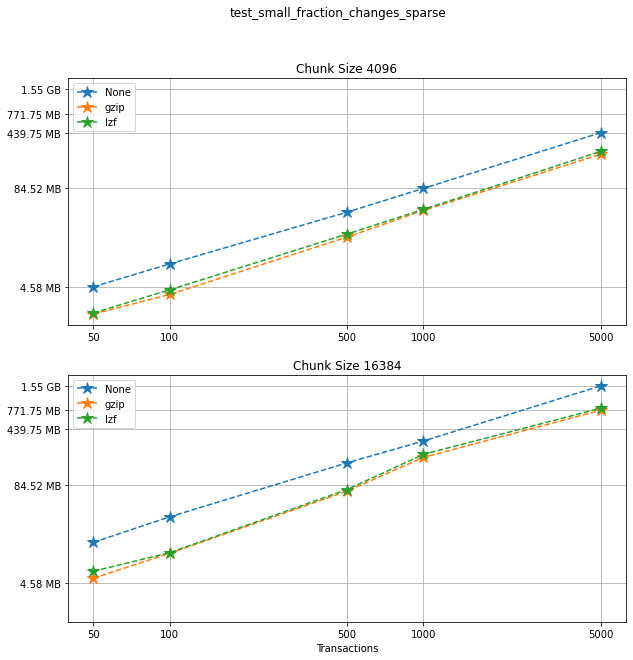
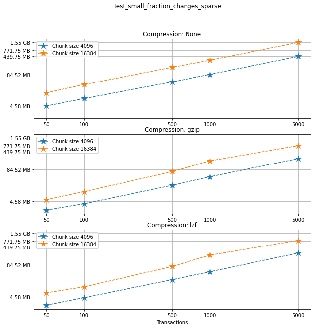
Comparing chunk sizes

Now, for each choice of compression algorithm, we compare different chunk sizes.

fig, ax = plt.subplots(ncomp, figsize=(10,10), sharey=True)
fig.suptitle(f"{testname}: File sizes")

for i in range(ncomp):
    start = i*ncs*n
    for j in range(ncs):
        plotlabel = f"Chunk size {chunk_sizes[start+j*n]}"
        plottitle = f"Compression: {compression[start]}"
        ax[i].loglog(num_transactions[:n],
                     filesizes[start+j*n:start+(j+1)*n],
                     '*--', ms=12,
                     label=plotlabel)
        ax[i].legend(loc='upper left')
        ax[i].set_title(plottitle)
        ax[i].set_xticks(num_transactions[:n])
        ax[i].set_xticklabels(num_transactions[:n])
        ax[i].set_yticks(filesizes[selected])
        ax[i].set_yticklabels(sizelabels[selected])
        ax[i].grid(True)
        ax[i].minorticks_off()

plt.xlabel("Transactions")
plt.suptitle(f"{testname}")
plt.show()

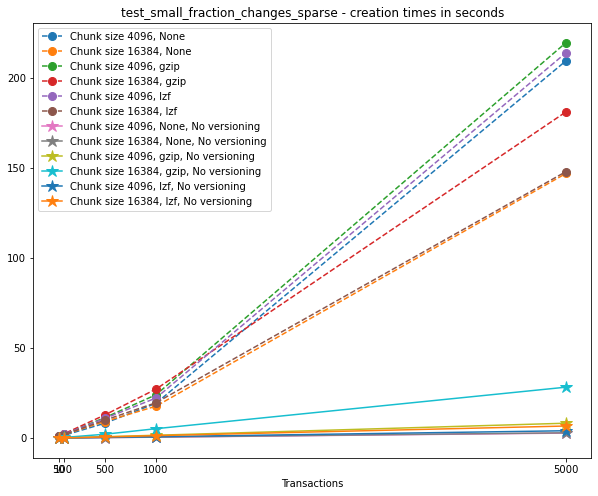
Creation times

If we look at the creation times for these files, we have something like this:

t_write = np.array([test['t_write'][-1] for test in testcase_3])
fig_large_fraction_changes_times = plt.figure(figsize=(10,8))
for i in range(ncomp):
    start = i*ncs*n
    for j in range(ncs):
        plt.plot(num_transactions[:n],
                 t_write[start+j*n:start+(j+1)*n],
                 'o--', ms=8,
                 label=f"Chunk size {chunk_sizes[start+j*n]}, {compression[start]}")

# If you also with to plot information about the "no versions" test,
# run the following lines:
t_write_nv = np.array([test['t_write'][-1] for test in testcase_3_no_versions])
for i in range(ncomp):
    start = i*ncs*n
    for j in range(ncs):
        plt.plot(num_transactions[:n],
                 t_write_nv[start+j*n:start+(j+1)*n],
                 '*-', ms=12,
                 label=f"Chunk size {chunk_sizes[start+j*n]}, {compression[start]}, No versioning")

plt.xlabel("Transactions")
plt.title(f"{testname} - creation times in seconds")
plt.legend()
plt.xticks(num_transactions[:n])
plt.show()

Again, the graphs below show, for each fixed number of transactions, the time required to add new versions as the file is created.

fig_times, ax = plt.subplots(n+1, figsize=(14,20))
fig_times.suptitle(f"{testname}: time to write each new version")

for i in range(n):
    for test in testcase_3:
        if test['num_transactions'] == num_transactions[i]:
            t_write = np.array(test['t_write'][:-1])
            ax[i].plot(t_write,
                       label=f"chunk size {test['chunk_size']}, {test['compression']}")
            ax[i].legend(loc='upper left')

# If you also with to plot information about the "no versions" test,
# run the following lines:
for test in testcase_3_no_versions:
    if test['num_transactions'] == num_transactions[i]:
        t_write = np.array(test['t_write'][:-1])
        ax[n].plot(t_write,
                   label=f"chunk size {test['chunk_size']}, {test['compression']}")
        ax[n].legend(loc='upper left')
        ax[n].set_title('No versioning')

plt.xlabel("Number of transactions")
plt.ylabel("Time (in seconds)")
plt.show()

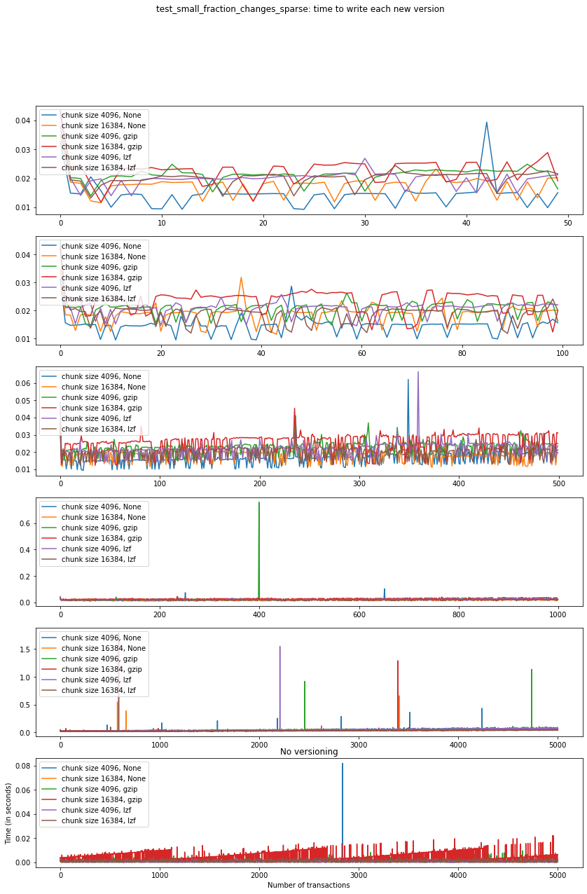
Summary

This behaviour is very similar to what we got in the test_large_fraction_changes_sparse case, with the exception that the times required to write new versions to the file are on average smaller than those in the former case. This is expected both in the versioned and unversioned case.

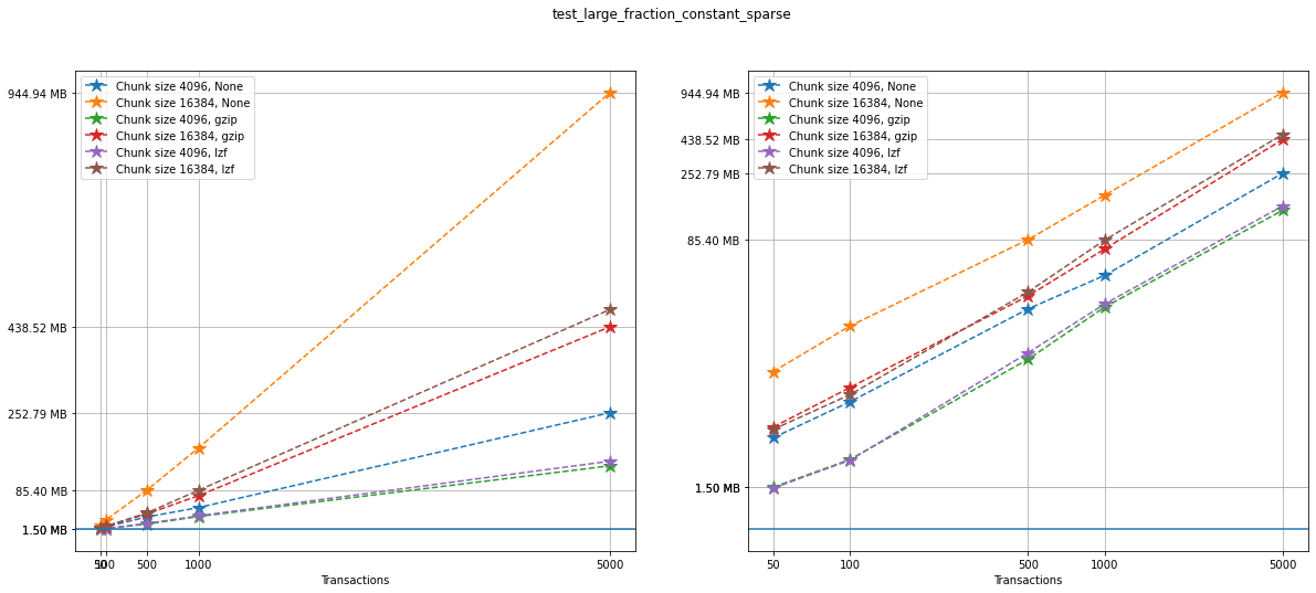
Test 4: Large fraction changes - constant array size (sparse)

testname = "test_large_fraction_constant_sparse"

We have tested the following options:

num_transactions_4 = [50, 100, 500, 1000, 5000]
exponents_4 = [12, 14]
compression_4 = [None, "gzip", "lzf"]

Analysis

Again, let’s show the size information in a graph:

num_transactions = [test['num_transactions'] for test in testcase_4]
chunk_sizes = [test['chunk_size'] for test in testcase_4]
compression = [test['compression'] for test in testcase_4]
filesizes = np.array([test['size'] for test in testcase_4])
sizelabels = np.array([test['size_label'] for test in testcase_4])
max_no_versions = max(np.array([test['size'] for test in testcase_4_no_versions]))

n = len(set(num_transactions))
ncs = len(set(chunk_sizes))
ncomp = len(set(compression))

Again, on the left we can see a linear plot, and on the right a loglog plot of the same size data for testcase_4. A blue solid horizontal line indicates the maximum file size obtained when generating the same tests with no versioning (that is, not using VersionedHDF5).

fig, ax = plt.subplots(nrows=1, ncols=2, figsize=(20,8))

selected = [10, 4, 7, 9, 10, 19]

for i in range(ncomp):
    start = i*ncs*n
    for j in range(ncs):
        ax[0].plot(num_transactions[:n],
                   filesizes[start+j*n:start+(j+1)*n],
                   '*--', ms=12,
                   label=f"Chunk size {chunk_sizes[start+j*n]}, {compression[start]}")
        ax[1].loglog(num_transactions[:n],
                     filesizes[start+j*n:start+(j+1)*n],
                     '*--', ms=12,
                     label=f"Chunk size {chunk_sizes[start+j*n]}, {compression[start]}")
        ax[0].legend(loc='upper left')
        ax[1].legend(loc='upper left')
        ax[0].minorticks_off()
        ax[1].minorticks_off()
        # Changing the indices in selected will change the y-axis ticks in the graph for better visualization
        ax[0].set_xticks(num_transactions[:n])
        ax[0].set_xticklabels(num_transactions[:n])
        ax[0].set_yticks(filesizes[selected])
        ax[0].set_yticklabels(sizelabels[selected])
        ax[0].set_xlabel("Transactions")
        ax[0].grid(True)
        ax[1].set_xticks(num_transactions[:n])
        ax[1].set_xticklabels(num_transactions[:n])
        ax[1].set_yticks(filesizes[selected])
        ax[1].set_yticklabels(sizelabels[selected])
        ax[1].set_xlabel("Transactions")
        ax[1].grid(True)

ax[0].axhline(max_no_versions)
ax[1].axhline(max_no_versions)
plt.suptitle(f"{testname}")
plt.show()

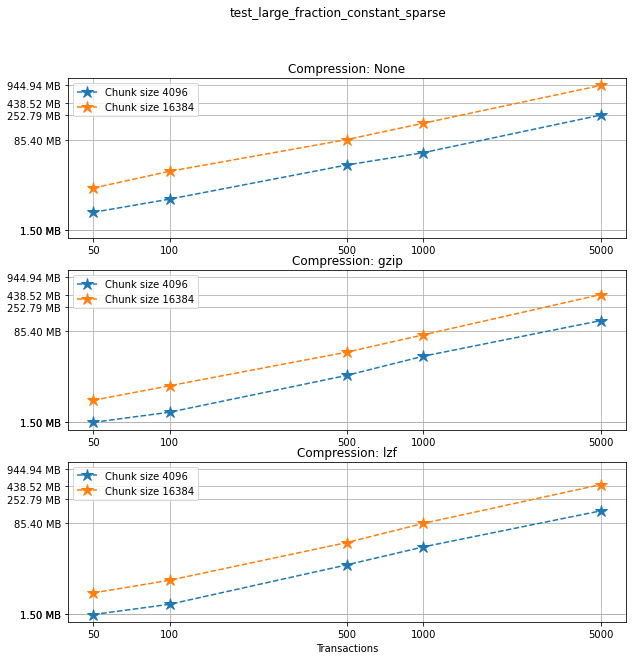
Comparing compression algorithms

For each chunk size that we chose to test, let’s compare the file sizes corresponding to each compression algorithm that we used.

fig, ax = plt.subplots(ncs, figsize=(10,10), sharey=True)
fig.suptitle(f"{testname}: File sizes")

for i in range(ncomp):
    start = i*ncs*n
    for j in range(ncs):
        ax[j].loglog(num_transactions[:n],
                     filesizes[start+j*n:start+(j+1)*n],
                     '*--', ms=12,
                     label=f"{compression[start]}")
        ax[j].legend(loc='upper left')
        ax[j].set_title(f"Chunk Size {chunk_sizes[start+j*n]}")
        ax[j].set_xticks(num_transactions[:n])
        ax[j].set_xticklabels(num_transactions[:n])
        ax[j].set_yticks(filesizes[selected])
        ax[j].set_yticklabels(sizelabels[selected])
        ax[j].grid(True)
        ax[j].minorticks_off()

plt.xlabel("Transactions")
plt.suptitle(f"{testname}")
plt.show()

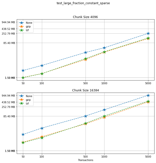
Comparing chunk sizes

Now, for each choice of compression algorithm, we compare different chunk sizes.

fig, ax = plt.subplots(ncomp, figsize=(10,10), sharey=True)
fig.suptitle(f"{testname}: File sizes")

for i in range(ncomp):
    start = i*ncs*n
    for j in range(ncs):
        plotlabel = f"Chunk size {chunk_sizes[start+j*n]}"
        plottitle = f"Compression: {compression[start]}"
        ax[i].loglog(num_transactions[:n],
                     filesizes[start+j*n:start+(j+1)*n],
                     '*--', ms=12,
                     label=plotlabel)
        ax[i].legend(loc='upper left')
        ax[i].set_title(plottitle)
        ax[i].set_xticks(num_transactions[:n])
        ax[i].set_xticklabels(num_transactions[:n])
        ax[i].set_yticks(filesizes[selected])
        ax[i].set_yticklabels(sizelabels[selected])
        ax[i].grid(True)
        ax[i].minorticks_off()

plt.xlabel("Transactions")
plt.suptitle(f"{testname}")
plt.show()

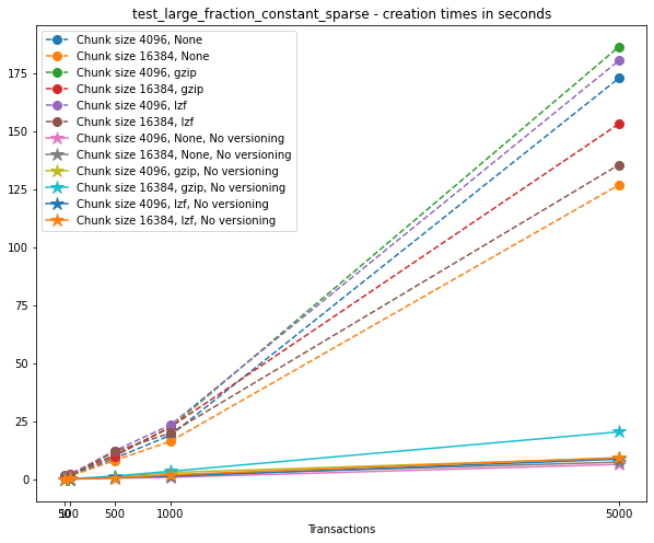
Creation times

If we look at the creation times for these files, we have something like this:

t_write = np.array([test['t_write'][-1] for test in testcase_4])
fig_large_fraction_changes_times = plt.figure(figsize=(10,8))
for i in range(ncomp):
    start = i*ncs*n
    for j in range(ncs):
        plt.plot(num_transactions[:n],
                 t_write[start+j*n:start+(j+1)*n],
                 'o--', ms=8,
                 label=f"Chunk size {chunk_sizes[start+j*n]}, {compression[start]}")

# If you also with to plot information about the "no versions" test,
# run the following lines:
t_write_nv = np.array([test['t_write'][-1] for test in testcase_4_no_versions])
for i in range(ncomp):
    start = i*ncs*n
    for j in range(ncs):
        plt.plot(num_transactions[:n],
                 t_write_nv[start+j*n:start+(j+1)*n],
                 '*-', ms=12,
                 label=f"Chunk size {chunk_sizes[start+j*n]}, {compression[start]}, No versioning")

plt.xlabel("Transactions")
plt.title(f"{testname} - creation times in seconds")
plt.legend()
plt.xticks(num_transactions[:n])
plt.show()

Again, the graphs below show, for each fixed number of transactions, the time required to add new versions as the file is created.

fig_times, ax = plt.subplots(n+1, figsize=(14,20))
fig_times.suptitle(f"{testname}: time to write each new version")

for i in range(n):
    for test in testcase_4:
        if test['num_transactions'] == num_transactions[i]:
            t_write = np.array(test['t_write'][:-1])
            ax[i].plot(t_write,
                       label=f"chunk size {test['chunk_size']}, {test['compression']}")
            ax[i].legend(loc='upper left')

# If you also with to plot information about the "no versions" test,
# run the following lines:
for test in testcase_4_no_versions:
    if test['num_transactions'] == num_transactions[i]:
        t_write = np.array(test['t_write'][:-1])
        ax[n].plot(t_write,
                   label=f"chunk size {test['chunk_size']}, {test['compression']}")
        ax[n].legend(loc='upper left')
        ax[n].set_title('No versioning')

plt.xlabel("Number of transactions")
plt.ylabel("Time (in seconds)")
plt.show()

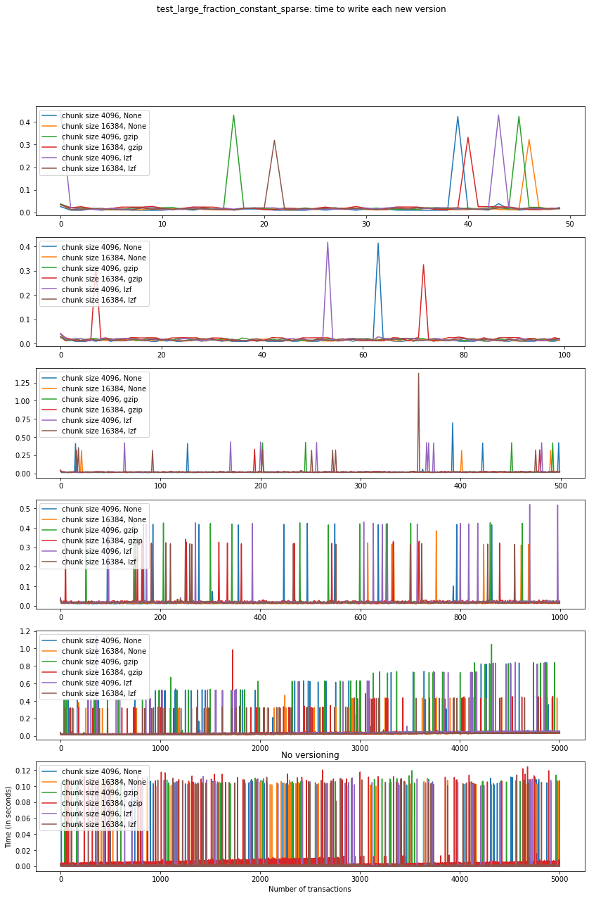
This behaviour is again very similar to test_large_fraction_changes, except that we don’t see the tendency to have larger times required to add new versions as the number of transactions grows.

Test 5: Mostly appends (dense)

testname = "test_mostly_appends_dense"

Note that this case includes a two-dimensional dataset. For this reason, we have chosen different chunk sizes to test, considering that larger chunk sizes increase file sizes considerably in this case.

For this case, we have tested the following options:

num_transactions_5 = [25, 50, 100, 500]
exponents_5 = [6, 8, 10]
compression_5 = [None, "gzip", "lzf"]

Analysis

Let’s show the size information in a graph:

num_transactions = [test['num_transactions'] for test in testcase_5]
chunk_sizes = [test['chunk_size'] for test in testcase_5]
compression = [test['compression'] for test in testcase_5]
filesizes = np.array([test['size'] for test in testcase_5])
sizelabels = np.array([test['size_label'] for test in testcase_5])
max_no_versions = max(np.array([test['size'] for test in testcase_5_no_versions]))

n = len(set(num_transactions))
ncs = len(set(chunk_sizes))
ncomp = len(set(compression))

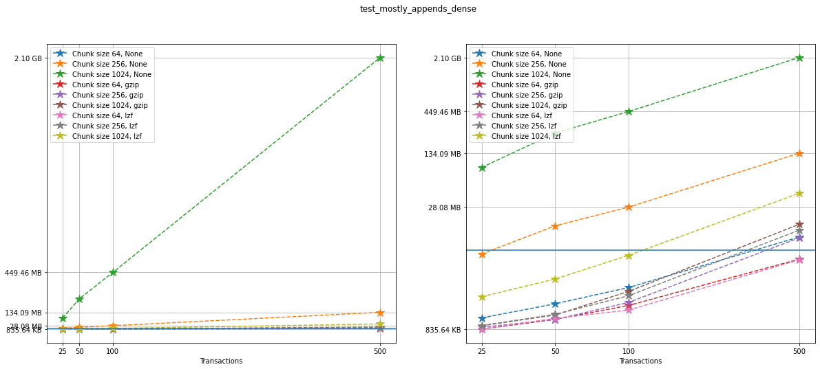
Once more, on the left we can see a linear plot, and on the right a loglog plot of the same size data for testcase_5. A blue solid horizontal line indicates the maximum file size obtained when generating the same tests with no versioning (that is, not using VersionedHDF5).

fig, ax = plt.subplots(nrows=1, ncols=2, figsize=(20,8))

selected = [6, 7, 10, 11, 12]

for i in range(ncomp):
    start = i*ncs*n
    for j in range(ncs):
        ax[0].plot(num_transactions[:n],
                   filesizes[start+j*n:start+(j+1)*n],
                   '*--', ms=12,
                   label=f"Chunk size {chunk_sizes[start+j*n]}, {compression[start]}")
        ax[1].loglog(num_transactions[:n],
                     filesizes[start+j*n:start+(j+1)*n],
                     '*--', ms=12,
                     label=f"Chunk size {chunk_sizes[start+j*n]}, {compression[start]}")
        ax[0].legend(loc='upper left')
        ax[1].legend(loc='upper left')
        ax[0].minorticks_off()
        ax[1].minorticks_off()
        # Changing the indices in selected will change the y-axis ticks in the graph for better visualization
        ax[0].set_xticks(num_transactions[:n])
        ax[0].set_xticklabels(num_transactions[:n])
        ax[0].set_yticks(filesizes[selected])
        ax[0].set_yticklabels(sizelabels[selected])
        ax[0].set_xlabel("Transactions")
        ax[0].grid(True)
        ax[1].set_xticks(num_transactions[:n])
        ax[1].set_xticklabels(num_transactions[:n])
        ax[1].set_yticks(filesizes[selected])
        ax[1].set_yticklabels(sizelabels[selected])
        ax[1].set_xlabel("Transactions")
        ax[1].grid(True)

ax[0].axhline(max_no_versions)
ax[1].axhline(max_no_versions)
plt.suptitle(f"{testname}")
plt.show()

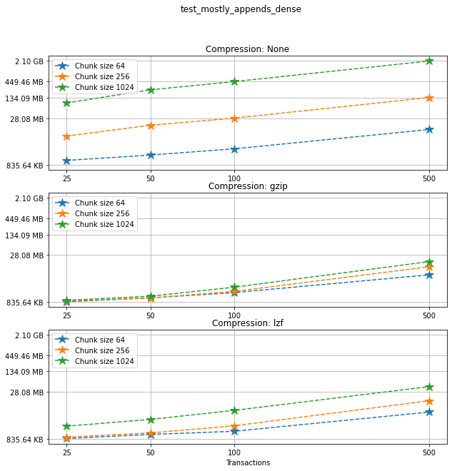
Comparing compression algorithms

For each chunk size that we chose to test, let’s compare the file sizes corresponding to each compression algorithm that we used.

fig, ax = plt.subplots(ncs, figsize=(10,10), sharey=True)
fig.suptitle(f"{testname}: File sizes")

for i in range(ncomp):
    start = i*ncs*n
    for j in range(ncs):
        ax[j].loglog(num_transactions[:n],
                     filesizes[start+j*n:start+(j+1)*n],
                     '*--', ms=12,
                     label=f"{compression[start]}")
        ax[j].legend(loc='upper left')
        ax[j].set_title(f"Chunk Size {chunk_sizes[start+j*n]}")
        ax[j].set_xticks(num_transactions[:n])
        ax[j].set_xticklabels(num_transactions[:n])
        ax[j].set_yticks(filesizes[selected])
        ax[j].set_yticklabels(sizelabels[selected])
        ax[j].grid(True)
        ax[j].minorticks_off()

plt.xlabel("Transactions")
plt.suptitle(f"{testname}")
plt.show()

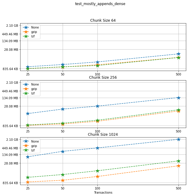
Comparing chunk sizes

Now, for each choice of compression algorithm, we compare different chunk sizes.

fig, ax = plt.subplots(ncomp, figsize=(10,10), sharey=True)
fig.suptitle(f"{testname}: File sizes")

for i in range(ncomp):
    start = i*ncs*n
    for j in range(ncs):
        plotlabel = f"Chunk size {chunk_sizes[start+j*n]}"
        plottitle = f"Compression: {compression[start]}"
        ax[i].loglog(num_transactions[:n],
                     filesizes[start+j*n:start+(j+1)*n],
                     '*--', ms=12,
                     label=plotlabel)
        ax[i].legend(loc='upper left')
        ax[i].set_title(plottitle)
        ax[i].set_xticks(num_transactions[:n])
        ax[i].set_xticklabels(num_transactions[:n])
        ax[i].set_yticks(filesizes[selected])
        ax[i].set_yticklabels(sizelabels[selected])
        ax[i].grid(True)
        ax[i].minorticks_off()

plt.xlabel("Transactions")
plt.suptitle(f"{testname}")
plt.show()

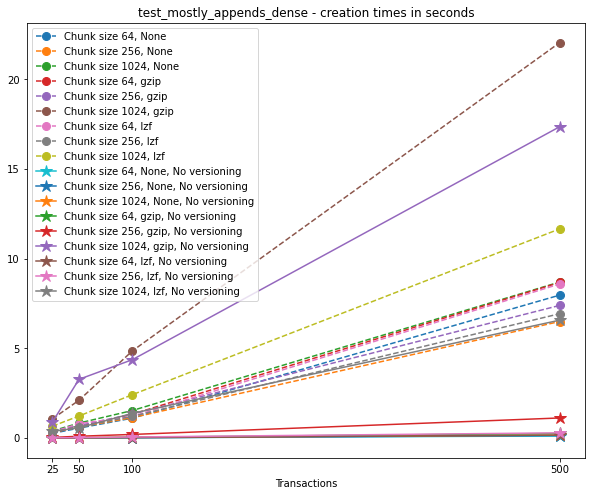
Creation times

If we look at the creation times for these files, we have something like this:

t_write = np.array([test['t_write'][-1] for test in testcase_5])
fig_large_fraction_changes_times = plt.figure(figsize=(10,8))
for i in range(ncomp):
    start = i*ncs*n
    for j in range(ncs):
        plt.plot(num_transactions[:n],
                 t_write[start+j*n:start+(j+1)*n],
                 'o--', ms=8,
                 label=f"Chunk size {chunk_sizes[start+j*n]}, {compression[start]}")

# If you also with to plot information about the "no versions" test,
# run the following lines:
t_write_nv = np.array([test['t_write'][-1] for test in testcase_5_no_versions])
for i in range(ncomp):
    start = i*ncs*n
    for j in range(ncs):
        plt.plot(num_transactions[:n],
                 t_write_nv[start+j*n:start+(j+1)*n],
                 '*-', ms=12,
                 label=f"Chunk size {chunk_sizes[start+j*n]}, {compression[start]}, No versioning")

plt.xlabel("Transactions")
plt.title(f"{testname} - creation times in seconds")
plt.legend()
plt.xticks(num_transactions[:n])
plt.show()

Again, the graphs below show, for each fixed number of transactions, the time required to add new versions as the file is created.

fig_times, ax = plt.subplots(n+1, figsize=(14,20))
fig_times.suptitle(f"{testname}: time to write each new version")

for i in range(n):
    for test in testcase_5:
        if test['num_transactions'] == num_transactions[i]:
            t_write = np.array(test['t_write'][:-1])
            ax[i].plot(t_write,
                       label=f"chunk size {test['chunk_size']}, {test['compression']}")
            ax[i].legend(loc='upper left')

# If you also with to plot information about the "no versions" test,
# run the following lines:
for test in testcase_5_no_versions:
    if test['num_transactions'] == num_transactions[i]:
        t_write = np.array(test['t_write'][:-1])
        ax[n].plot(t_write,
                   label=f"chunk size {test['chunk_size']}, {test['compression']}")
        ax[n].legend(loc='upper left')
        ax[n].set_title('No versioning')

plt.xlabel("Number of transactions")
plt.ylabel("Time (in seconds)")
plt.show()

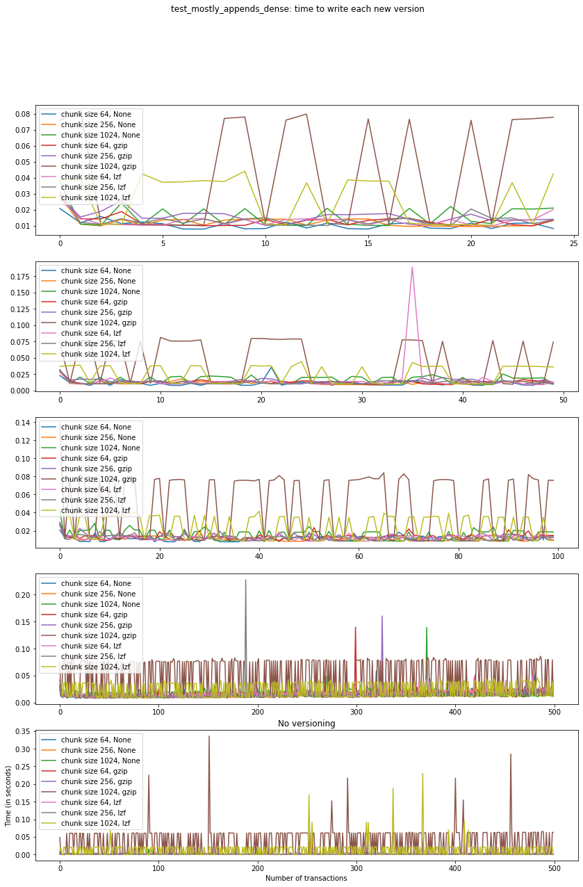
Summary

This test case is unique for a few reasons. First, having a two-dimensional dataset introduces new considerations, such as the number of rows being added in each axis. For this test case, we have only added (few) new rows to the first axis with each new version, and this might explain why we don’t see an increase in the time required to write new versions to file as the number of transactions grow. In addition, we can see that in the case of 500 transactions, the creation of the unversioned file can also take a hit in performance. These are preliminary tests, and multidimensional datasets are still experimental at this point in VersionedHDF5.